Chapter 9 Fitting a dynamic transmission model of Tuberculosis

9.1 Introduction

In the previous chapter I outlined a mechanistic model of Tuberculosis (TB) transmission. Whilst this model made use of the best available evidence there remains a large degree of uncertainty regarding it’s structure and parameterisation. The majority of this uncertainty relates to the amount of TB transmission occurring in England. In order to use this model to understand TB transmission, and the impact of different BCG vaccination policies (Chapter 10) this uncertainty needs to be reduced and the parameter space tightened to reflect more realistic ranges. An approach to deal with this uncertainty is to fit the model to available observed data. Model fitting involves optimising over the available parameter space to return parameter sets that fit the data in some quantitative way “better” than other parameter sets. An alternative to model fitting is using a model parameterised with expert knowledge only for inference. This approach is not appropriate here due to the large amount of uncertainty for many of the model parameters. Any inference based on just the parametisation from the previous chapter would have large credible intervals, reflect reality poorly, and likely be biased in multiple areas.

This chapter details an approach to fitting a infectious disease model to data using the state-space model formulation and Bayesian model fitting techniques. It first outlines the infectious disease model discussed in the previous chapter as a state-space model, as well as detailing the data used for fitting the model, the parameters that are fitted, and the parameters that are modelled stochastically. It then outlines the theoretical, and practical, justification for the model fitting pipeline used to calibrate and fit this state space model. Finally it discusses the quality of the model fit, ad hoc techniques used to improve model fit, strengths and limitations of the approach, and areas for further work.

9.2 Formulation as a state-space models

State space models (SSMs) may be used to model dynamic systems that are partially observed (such as all but the most contained infectious disease outbreak or endemic). They consist of a set of parameters, a latent continuous/discrete time state process and an observed continuous/discrete time process.[123] The model developed in the previous section represents the state process of the SSM, with the parameters estimated for the model representing the model initial conditions and parameter set. To complete the mapping to an SSM an observational model is required. This observational model takes the latent estimates from the dynamic model and forecasts the observed data. I specify such an observational model in Section 9.2.2.

9.2.1 Observed data

The primary data source for the model is the reported, age-stratified, UK born TB notifications from 2000 to 2004 as recorded in the Enhanced TB Surveillance (ETS) system (see Chapter 4). 2000 to 2004 are the years for which notifications are stratified by UK birth status with universal school-age BCG vaccination. Data were grouped using the age groups present in the dynamic model (5 year age groups up to 49 and then a group from 50-69 and a 70+ group). Using age-stratified incidence data, versus aggregated data, allows for more complex trends to be identified. Non-UK born TB notifications were extracted from the same source for use as an input to the models force of infection (Chapter 8).

Additional datasets were considered during initial model fitting and during later model calibration. These were a condensed version of the age stratified data discussed above with a reduced number of age groups (children (aged 0-14 years old), adults (15-69 years old), and older adults (70-89 years old)) and a dataset of historic pulmonary TB notifications. The advantage of condensing age groups was that the number of notifications in each group increased. This reduced the impact of stochastic noise, making fitting the model easier as trends in the data are more consistent. Secondly, reducing the number of data points, whilst still capturing the important age dynamics, reduces the compute requirements of the model (see Section 9.3.1). As will be discussed in Section 9.3 this was a major consideration as the model fitting approach used was highly compute intensive. The downside of this approach is that potentially important information may be lost when data is condensed into fewer groups. Historic pulmonary TB notifications (including both UK born and non-UK born cases) from 1990, 1994, and 1998 were considered as using data from the decade prior to the time period of interest allows the long term trends to be fitted to. A subset of the available data was used as this limited the impact on the compute time of the fitting pipeline. These data were originally collected in the Statutory Notifications of Infectious Diseases (NOIDS) dataset with notifications from 1913 to 1999. These data were sourced from Public Health England,[2] and made available in R using tbinenglanddataclean³¹. Downsides of using these data are that reporting standards may have changed over time so a single measurement model may not be appropriate and non-UK born cases are included in these data making fitting to this data dependent on the number of non-UK born cases pre 2000 which are themselves estimated during model fitting.

9.2.2 Observational model

There are three major considerations to account for when developing an observed disease notification model (i.e a reporting model). These are: systematic reporting error over time; systematic changes in reporting error over time; and reporting noise. I assumed that all reporting errors are Gaussian and that there are no time variable reporting errors. This model was used for all data fitted to. The reporting model can be defined as follows,

\[O = \mathcal{N}\left(E_{\text{syst}}A, E_{\text{noise}}A\right)\]

Where \(O\) are the observed notifications, \(A\) are the incident cases of disease as forecast by the disease transmission model, \(E_{\text{syst}}\) is the systematic reporting error, \(E_{\text{noise}}\) is the reporting noise, and \(\mathcal{N}\) represents the Gaussian (normal) distribution. The priors for the model are defined in Table 9.1. The prior for systematic reporting error is based on the assumption that underreporting is more likely than over-reporting. The prior for the reporting noise is based on the observed variation between years. This observation model is also used when incorporating non-UK born incidence rates into the models force of infection (Chapter 8). This allows the uncertainty in these observations to be properly accounted for in the incidence estimates produced by the fitted model.

A potential limitation of this model is that reporting of TB cases is likely to have improved over time. This is especially true of notifications reported prior to the introduction of the ETS in 2000. A potential improvement to this model would be to introduce separate systematic reporting errors for notifications pre- and post- the introduction of the ETS. However, this may result in over-fitting and so has not been implemented here.

Table 9.1: Measurement model parameters, descriptions, prior distributions, units, method used to derive the prior distribution and the type (i.e data derived, literature, assumption). \(\mathcal{U}\) = Uniform

Parameter	Description	Distribution	Units	Method	Type
\(E_{\text{syst}}\)	Systematic reporting error of incident TB cases	\(\mathcal{N}(0.9, 0.05)\) truncated to be greater than 0.8 and lower than 1.	Proportion	Assumption is that underreporting of TB cases is likely with no overreporting.	Assumption
\(E_{\text{noise}}\)	Magnitude of reporting noise for incidence TB cases.	\(\mathcal{U}(0, 0.025)\).	Proportion	It is likely that reporting accuracy varies each year. An upper bound of 2.5% is used as this means that approximately 95% of observations will be within 10% of each other.	Assumption

9.2.3 Fitted parameters

The model outlined in Chapter 8 has a large number of free parameters for which prior distributions have been specified based on the observed data, the literature, and expert knowledge. In theory the model fitting pipeline outlined below could be used to produce posterior distributions for all these parameters. However, in practice this is not feasible as the data discussed in Section 9.2.1 only covers notifications and therefore does not contain sufficient information. If every parameter was allowed to update based on the data then it is likely that the resulting posterior distributions would not match with alternative data sources and the literature. Another potential issue is that by allowing all parameters to be fitted the meaningful transmission related information in the observed data may be lost due to over-fitting from other variables.

For this reason in the model fitting pipeline outlined here I have only allowed parameters relating to TB transmission, and measurement model parameters, to have their posterior distributions updated by the model fitting pipeline. All other parameters have posterior distributions that match their prior distributions. Parameters that have updated posterior distributions based on the data are,

• Mixing rate between UK born and non-UK born (\(M\)).
• Scaling on non-UK born cases (\(\iota_{\text{scale}}\)).
• Effective contact rate (\(c_{\text{eff}}\)).
• Historic effective contact rate (\(c^{\text{hist}}_{\text{eff}}\)).
• Half life of the effective contact rate (\(c^{\text{hist}}_{\text{half}}\)).
• Low risk latent activation rate modifier for older adults (70+) (\(\epsilon^{\text{older-adult}}_L\)).
• Systematic reporting error (\(E_{\text{syst}}\)).
• Reporting noise (\(E_{\text{noise}}\)).

In addition for scenarios with age variable transmission probabilities or non-UK born mixing the following parameters may also be fitted to,

• Transmission probability modifier for young adults (\(\beta_{\text{young adult}}\)).
• Non-UK born mixing modifier for young adults (\(M_{\text{young adult}}\)).

9.2.4 Stochastic parameters

Several key data inputs such as incidence in the non-UK born population, coverage of the BCG vaccination program, births, deaths and the contact rate are not perfectly observed, or recorded, and may vary across time. For these reasons, these parameters are included in the model developed in the last chapter as noise terms. This means that they are resampled for each timestep and so vary stochastically over time. This results in a model that is semi-stochastic rather than being fully deterministic (Chapter 1). A semi-stochastic model can be defined as a deterministic model that incorporates stochastic elements but that is still solved as a deterministic system within a given timestep. It is a modelling approach that has been used previously in the literature when key parameters are uncertain and potentially time-varying.[9] For further details of the stochastic parameters included in the model see Chapter 8.

9.3 Model fitting pipeline

Fitting dynamic transmission models is complex and requires the use of specialist statistical techniques. There are a variety of these tools available. Ranging from tried and tested to cutting edge. Historically many modellers have used maximum likelihood methods to fit deterministic models. More recently Bayesian methods have become popular. These have numerous benefits including: explicit inclusion of prior knowledge via prior distributions for all parameters; ability to handle complex stochastic models; and provide parameter distributions (posterior distribution) of best fitting parameters rather than single point estimates (or interval estimates).[123] Unfortunately, many of these methods also require tuning prior to use. This section outlines the theoretical justification, and implementation details, of an automated model fitting pipeline used to fit the previously detailed state space model.

LibBi was used for all model fitting.[123] LibBi is a software package for state-space modelling and Bayesian inference. It uses a domain specific language for model specification, which is then optimised and compiled to provide highly efficient model code. It focuses on full information model fitting approaches including: particle Markov chain Monte Carlo (PMCMC), and SMC-SMC methods for parameter estimation. All fitting algorithms are highly efficient and scalable across multiple CPUs or GPUs. The rbi and rbi.helpers packages were used to interface with LibBi from R.[124,125] rbi.helpers was also used to optimise the model fitting pipeline as detailed in the calibration section. As model fitting using LibBi is compute intensive a workstation was built, and overclocked (using CPU voltage manipulation), with these compute requirements in mind³². Whilst a cluster was theoretically available, in practise the hardware available was limited, installing LibBi was challenging, and run times were constrained by fair access. All model fitting code is available on GitHub as an R package³³.

9.3.1 The particle filter

In order to fit a model to data it is necessary to estimate, or calculate, the marginal likelihood. Mathematically, the marginal likelihood is the plausibility that a parameter set, given the specified statistical model and the initial conditions, describes the observed data. For complex state space models, such as that discussed in the previous chapter, calculating the marginal likelihood is not possible.[123] The particle filter provides a model-agnostic approach, based on importance sampling, to estimate the marginal likelihood. The variant used in this thesis, the bootstrap particle filter, is described below. See [123] for a more technical discussion of the bootstrap particle filter.

1. Sampling: For a given parameter set, the particle filter is initialised by drawing a number of random samples (state particles) from the initial conditions of the model under consideration. These samples are then given a uniform weighting.

2. Sequentially for the each observed data point, the particle filter is then advanced through a series of propagation, weighting, and re-sampling steps.

• Propagation: For each particle the model is simulated, producing a forecast of the observed data point.

• Weighting: The likelihood of the new observation, given the predicted state, is then computed for each state particle. State particles are then weighted based on this likelihood.

• Re-sampling: The particle stocke is restorted to equal weights by re-sampling particles, with replacement, with the probability of each sample being drawn being proportional to it’s weight.

3. The marginal likelihood (likelihood of the observed data given the parameter set, marginalised across the initial conditions) can then be estimated by taking the product of the mean likelihood at each observed data point. A sample trajectory can also be calculated using the estimated weights from each time point.

9.3.2 Sequential Monte Carlo

The particle filter approach outlined above, is a member of a family of sequential Monte Carlo (SMC) methods. These methods all initialise particles and then follow the same propagation, weighting, and re-sampling steps as previously detailed. SMC may also be used to sample from the posterior distribution of a given set of priors and a specified model. This works as follows,

1. Initially a number of samples (parameter particles) is taken from the prior distribution of the parameters and assigned a uniform weighting.

2. These parameter particles are then iterated sequentially over each observed data point, undergoing the same propagation, weighting, and re-sampling steps as in the particle filter, as well as an additional rejuvenation step.

   • Propagation: The model is simulated to the next observed data point.

   • Weighting: Parameter particles are weighted using the marginal likelihood. In principle this could be computed exactly, but is most commonly estimated using a nested particle filter for each state particle (i.e as outlined in the previous section). For a subset of models, a Kalman filter may be used instead.[123] The marginal likelihood may also be estimated using other partial information techniques such as approximate Bayesian computation. In the case where a particle filter is used the full algorithm is known as Sequential Monte Carlo - Sequential Monte Carlo (SMC-SMC).[123] This algorithm is used for all dynamic model fitting in this thesis.

   • Re-sampling: The parameter particle stock is restored to equal weights by re-sampling particles, with replacement, with the probability of each sample being drawn being proportional to it’s weight.

   • Rejuvenation: Re-sampling of the parameter particles at each time point leads to a reduction in the number of unique values present. For state particles (when estimating the marginal likelihood using a particle filter) particles are diversified with each propagation but as parameters do not change in time parameter particles cannot diversify in this way. To account for this the rejuvenation step is inserted after the re-sampling of parameter particles at each time point. The rejuvenation step is a single, or multiple depending on the acceptance rate, Metropolis-Hastings step for each parameter particle. This step aims to preserve the distribution of the parameter particles, whilst increasing their diversity. To minimize unnecessary rejuvenation an effective sample size threshold can be used. This only triggers rejuvenation when particle diversity has decreased below the target effective sample size threshold.

9.3.2.1 Marginal Metropolis-Hastings

The Metropolis-Hasting step may be used as a model fitting approach in it’s own right (MCMC) when repeated sequentially. It works by proposing a new value from the proposal distribution, estimating the marginal likelihood using the attached particle filter (or using any other exact or inexact method), and then accepting or rejecting the move based on the acceptance probability.[123] Where the acceptance probability is given by,

\[ \text{min} \left(1, \frac{p(y(t_{1:T}) |\theta')p(\theta')q(\theta | \theta')}{p(y(t_{1:T}) |\theta)p(\theta)q(\theta' | \theta)}\right) \]

Where \(y\) is the observed data, \(\theta\) is the current parameter set, \(\theta'\) is some proposed parameter set sampled from some proposal distribution \(q(\theta' | \theta)\).[123] By construction, samples drawn using this rule are ergodic to the posterior distribution. This means that after convergence, samples drawn using this rule may be considered as samples from the posterior distribution.

9.3.3 Calibration

9.3.3.1 Particle calibration

The accuracy of the marginal likelihood estimate returned by the particle filter is dependent on the number of particles used, the number of observed data points, the parameter sample, and the complexity of the model. As the number of particles tends towards infinity the likelihood estimate provided by the particle filter should tend towards the exact solution. This suggests that choosing a very high number of particles may be the most efficient solution in terms of accuracy. Unfortunately, each particle requires a full model simulation, which for complex models can be computationally costly. This means that using very large numbers of particles is not tractable. For this reason it is necessary to determine an optimal number of particles that both provides an adequately accurate estimate of the likelihood whilst being computationally tractable.

The rbi.helpers R package attempts to solve this issue by adopting the following strategy.[125] First, the approximate mean of the posterior distribution is obtained, as accurate likelihood estimates near the posterior mean are of the most interest. Repeated model simulations are then run using the same set of parameters, with the marginal likelihood being estimated each time using a given number of particles. The variance of these log-likelihood estimates is then calculated. This process is then repeated for increasing numbers of particles until the log-likelihood variance is below some target threshold, commonly 1.[125]

I have implemented this as a two step process for each fitted scenario. Firstly, I used the Nelder-Mead simplex method, via LibBi,[123] to find a parameter set that optimised the maximum likelihood. I then initialised a 1000 step PMCMC chain with this parameter set, using 1024 particles in the particle filter. I then used rbi.helpers,[125] as outlined above, to estimate the number of particles required to produce a log-likelihood variance of less than 1 for this sample of the posterior distribution, using 250 samples per step and starting with 16 particles. I initially planned to repeat this process for multiple draws from the posterior distribution but this proved to be in-feasible given the compute available. A target of 5 for the log-likelihood variance was chosen as a smaller target could not be feasibly achieved given the compute resources available. Additionally 1024 was specified as the maximum number of feasible particles to use in the particle filter.

9.3.3.2 Proposal calibration

When using an MCMC algorithm a proposal distribution is required to provide new parameter samples to evaluate. For SMC-SMC a proposal distribution is required to inform the MCMC sampler that is run during the rejuvenation step. By default if no proposal distribution is provided LibBi uses the prior distribution.[123] The prior distribution can be an inefficient proposal distribution as it is likely to have a low acceptance rate (from the MCMC sampler).[123] Having a low acceptance rates means that many more MCMC steps are required to generate a successful parameter sample. This results in slow mixing and computationally expensive MCMC steps may make model fitting intractable.

A more efficient approach is to specify a proposal distribution that draws parameter samples that are closer to the current state of the MCMC chain than the overall prior distribution. There is an extensive literature examining how to optimise the proposal distribution to achieve an good acceptance rate. In practice it has been shown that a rate of between 10% and 20% is optimal for upwards of 5 parameters.[123] This strikes a balance between allowing the chain to fully explore the posterior distribution whilst still being as efficient as possible.

A simple approach to setting the proposal is to run a series of MCMC steps and then calculate the acceptance rate. Based on the acceptance rate the width of the proposal distributions can then be adapted. By repeating these steps multiple times a proposal distribution which gives an acceptance rate within the desired bounds can be arrived at. This adaption can either be independent for each parameter or dependent (taking into account empirical correlations). The adapt_proposal function, from the rbi.helpers R package,[125] implements this approach and is used in this model fitting pipeline. In many models, parameters are likely to have strong correlations (i.e between UK and Non-UK born mixing rate and effective contact rate). In these scenarios, it is likely that a dependent strategy for adapting the proposal distribution will more efficiently explore the posterior distribution. However, the downside of adapting the proposal distribution using dependent methods is that the resulting proposal is highly complex, is computationally expensive to compute and may breakdown in some areas of the posterior distribution.

In this model fitting pipeline I have used a maximum of 5 iterations of, manual, independent proposal adaption, drawing 250 samples in each iteration, starting with Gaussian distributions for each parameter, truncated by the range of the prior, with the mean based on the current parameter value. The standard deviation for each parameter was assumed to be the standard deviation of the prior if it was Gaussian and otherwise assumed to be the range of the prior if it was uniform. For each iteration I halved the size of the standard deviation of each parameter. As for the particle calibration, I initially used a maximum likelihood method to provide a point estimate of the best fitting parameter set, followed by 1000 PMCMC steps, using a 1024 particle filter. This means that the proposal distribution is adapted near to the posterior mean rather than in the tails of the posterior distribution.

I chose to use manual independent proposal adaption methods for several reasons. Firstly, when developing this pipeline the approaches implemented in rbi.helpers produced multiple transient errors in other rbi and rbi.helpers code. Secondly, the resulting dependent proposal distribution was highly complex, slow to compute, and difficult to debug. Finally, for SMC-SMC efficient exploration of the proposal distribution is less important than when using MCMC alone as SMC-SMC is initialised with multiple samples from the prior distribution. This means that multiple local maximas can be efficiently explored regardless of the proposal distribution used. The MCMC rejuvenation step then serves to provide additional samples from these local maximas. Proposal adaption was only carried out for the main model scenario with all other scenarios using this proposal distribution.

9.3.4 Model comparison

In the previous chapter multiple scenarios were outlined, each of which could be valid based on theoretical considerations. The observed data can be used to identify which of these scenarios best reflects reality. This can be done using the deviance information criterion (DIC). The DIC is a hierarchical modeling generalization of the Akaike information criterion (AIC) and can be used to compare nested models.[126]

Smaller DIC values should indicate a better fit to data than larger DIC values. The DIC is composed of the deviance, which favours a good fit, and the effective number of parameters, which penalises over-fitting.[126] Unlike the AIC the DIC can be estimated using samples from the posterior distribution and so is more readily calculated for models estimated using Bayesian methods. It can be defined as,

\[ {\mathit {DIC}}=D({\bar {\theta }})+2p_{D}\] Where \(\bar{\theta}\) is the expectation of \(\theta\), with \(\theta\) being defined as the unknown parameters of the model. \(p_{D}\) is the effective number of parameters in the model and is used to penalise more complex models. It can be estimated as follows,[126]

\[p_{D}=p_{V}={\frac {1}{2}}\widehat {\operatorname {var}}\left(D(\theta )\right).\]

Finally the deviance is defined as,

\[D(\theta)=-2\log(p(y|\theta ))+C\]

Where y are the data, \(\displaystyle p(y|\theta)\) is the likelihood function and \(C\) is a constant. \(C\) cancels out when comparing different models and therefore does not need to be calculated.

The DIC has two limitations. The first of these is that in it’s derivation it is assumed that the model that generates future observations encompasses the true model. This assumption may not hold in all circumstances. The second limitations is that the observed data is used to construct both the posterior distribution and to estimate the DIC. This means that the DIC tends to select for over-fitted models.[126]

In this chapter I have used the DIC, as estimated by the DIC function from rbi.helpers,[125] to evaluate the various model structures outlined in the previous chapter.

9.3.5 Parameter sensitivity

Understanding the impact of parameter variation can help when interpreting findings from a model, targeting interventions, and identifying parameters for which improved estimates are needed. Often parameter sensitivity is assessed using single-parameter or local sensitivity analyses. Unfortunately, these techniques do not accurately capture uncertainty or sensitivity in the system as they hold all other parameters fixed.[127] Multiple techniques exist that can globally study a multi-dimensional parameter space but the partial rank correlation coefficient method (PRCC) that I will discuss, and implement, here has been shown to be both reliable and efficient.[127]

PRCC is a sampling based approach which can be computed with minimal computational cost from a sample of the prior or posterior distributions of a model. It estimates the degree of correlation between a given parameter input and an output after adjusting (using a linear model) for variation in other inputs. It is an extension of more simplistic sampling techniques, the most basic of which, is simply examining scatter plots of a sampled parameter set against the outcome of interest. PRCC is required as these more simplistic techniques become intractable with higher dimensionality as they do not account for between parameter correlation or are just difficult to interpret with multiple dimensions.[127] PRCC can be understod by first outlining the individual steps. These are:

1. Correlation: Provides a measure of the strength of a linear association between an input and and output (scaled from -1 to 1). It is calculated as follows,

\[ {\displaystyle \rho _{X,Y}={\frac {\operatorname {cov} (X,Y)}{\sigma _{X}\sigma _{Y}}}} \]

Where \(\operatorname {cov}\) is the covariance, \(\sigma _{X}\) is the standard deviation of \(X\), and \(\sigma_Y\) is the standard deviation of \(Y\). Where \(X\) is the input and \(Y\) is the output.

2. Rank Correlation: This is defined as for correlation but with the data being rank transformed. Rank transformation reorders inputs and outputs in magnitude order. Unlike non-rank transformed correlation it can handle non-linear relationships but still requires monotonicity.

3. Partial Rank Correlation: Inputs and outputs are first rank transformed as above. Linear models are then built which adjust for the effects of the other inputs on \(Y\), and on the current input \(X_i\). Correlation is the calculated as above using the residuals from these models.

A limitation of PRCC is that it whilst it can capture non-linear relationships between outputs and inputs these relationships must be monotonic.[127] For relationships that are non-monotic methods that rely on the decomposition of model output variance, such as the extended Fourier amplitude sensitivity test,[127] are more appropriate. However, these approaches are computationally demanding as they typically require multiple iterations of model simulation. Additionally, they cannot be used on a previous parameter samples, instead needing to sample and simulate the model within the parameter sensitivity algorithm. This means that they cannot be used for “free” (i.e with negligible additional compute cost), unlike PRCC which can be estimated using a sample from the posterior distribution. For this reason these approaches have not been further explored in this thesis.

I have implemented PRCC using the epiR R package³⁴,[60] using the samples from the posterior distribution of the model calculated during the SMC-SMC step. Parameter sensitivity measures such as PRCC must be calculated separately for each output time point. I calculated the PRCC for each fitted parameter, at the final time point with fitted data (2004), for overall TB incidence rates. These results are then summarised by plotting the absolute PRCC values, indicating the direction of correlation using colour³⁵.

9.3.6 Pipeline overview

The full model fitting pipeline can be summarised as follows³⁶:

1. Model initialisation using minimal error checking and single precision computation. Implemented using the disable-assert and enable-single flags in LibBi.[123] Outputs are only given for times with observed data and a subset of parameters are recorded for final reporting³⁷.

2. 1000 parameter sets were taken from the prior distribution and the model was then simulated for each one.

3. Maximum likelihood optimisation with 100 steps, using the Nelder-Mead simplex method, via LibBi.[123] This approximates the mean of the posterior distribution.

4. 1000 PMCMC steps, with 1024 particles used in the particle filter. This provides a better estimate of the mean of the posterior distribution.

5. Particle adaption via rbi.helpers at the approximate mean of the posterior distribution.[125] A minimum of 64 particles and a maximum of 1024 particles are assessed with the target of a log-likelihood variance of less than 5. 250 PMCMC steps were used at each stage to estimate the log-likelihood variance.

6. Manual independent proposal adaption at the approximate mean of the posterior distribution. It is assumed that the proposal for each parameter is Gaussian, truncated by the range of the prior with the mean based on the current parameter value. The standard deviation of the proposal distribution is halved each iteration, with at most 5 iterations of adaption. The minimum target acceptance rate specified was 10% and the maximum was 20%. 250 PMCMC samples were used each time to estimate the acceptance rate. Proposal adaption was only carried out for the main model scenario, with other scenarios using this proposal.

7. SMC-SMC model fitting with 1000 initial parameter particles. Particle rejuvenation was set to trigger when the effective sample size decreased below 25%, with 10 MCMC steps used each time.

8. For each sample from the posterior distribution the model was then simulated for all time points.

9. The model DIC was computed using rbi.helpers.[125] This gives a model agnostic approach to evaluate the fit to the observed data.

10. Parameter sensitivity was estimated by calculating the partial rank correlation coefficient (PRCC) for each model parameter, for the final time point fitted to (2004), for overall TB incidence rates. Results were then plotted in order of the absolute magnitude of the correlation, with the direction of the correlation determined using colour. The epiR package was used to compute the PRCC.[60]

9.4 Results

The pipeline outlined above resulted in a poor fit to the observed data. The SMC-SMC algorithm had a low effective sample size for each iteration, and a low acceptance rate for particle rejuvenation steps in all scenarios evaluated. This resulted in spuriously tight posterior distributions. Ad hoc calibration (detailed in the following section) failed to improve the quality of this fit or find a subset of the model - or parameters - that fit the observed data to an acceptable degree whilst remaining computationally feasible. All results presented in the following section are based on posterior distributions produced by the model fitting pipeline using the prior distributions specified in the previous chapter. The results are preliminary and indicative only.

9.4.1 Ad hoc calibration

Minor alterations to the model fitting pipeline had little impact on the quality of the fit. To attempt to improve the quality of the model fit I used a combination of ad hoc approaches. As a first step I introduced a calibration model with variation allowed only in the fitted parameters with all other parameters using point estimates. This allowed a reduced number of particles to be used to estimate the marginal likelihood and hence dramatically decreased compute cost and run-times. This reduced model was then used for the following tests:

• Increasing the number of particles used in the outer SMC loop at the expense of reducing the number of particles used for marginal likelihood estimation.
• Increasing the number of particles used for marginal likelihood estimation.
• Sequentially decreasing model complexity by fixing fitted parameters to manually tuned point estimates.
• Increasing the number of parameters fitted to rather than used as fixed distributions.
• Varying the size of the proposal distribution, rejuvenation threshold, number of particles and rejuvenation steps.
• Varying the fitted observed data. This took 3 main forms:
  • Aggregation: fitting to overall incidence only; fitting to incidence grouped by large age groups (i.e children, adults, older adults); fitting to only age groups of interest (i.e children).
  • Reducing the time-span of the fitted data. This included simplifying down to a single year of data but also included using various combinations of time points.
  • Exploring additional observed data. This included attempting to fit to observed pulmonary TB case from 1980 on-wards. This approach sought to constrain the parameter space to give a more realistic age distribution of cases.
• Changing the functional form for the decay in the historic contact rate. This involved exploring linear decay with the decay gradient dictated by the year that the current contact rate takes effect and the year that the historic contact rate began to decay.
• Exploring using time dependent modifiers on the transmission probability and non-UK born mixing.
• Exploring using modifiers for children, adults, and older adults for both the transmission probability and non-UK born mixing. This was essentially an extension of the original scenarios considered using the model fitting pipeline.
• Exploring widening and narrowing the prior distributions of fitted parameters beyond realistic ranges.
• Exploring varying the size of the initial high, and low risk latent populations. This included starting with no latent cases, starting with a reduced proportion of latent cases and starting with a much larger latent population to simulate a historically more widespread disease.

None of these approaches dramatically improved model fit to the point that more robust inference could be drawn. Reducing the number of parameters, and time points, fitted to decreased the computational cost of the pipeline and improved acceptance rates. However, model fits remained poor until a single time-point and aggregated incidence were fitted to using a single varying parameter (effective contact rate) with all others manually tuned. Unfortunately, this simplified the model to the extent that it could not be used to generate meaningful results. The introduction of multiple time-points led to poor model fits regardless of the observational data used. This effect may be attributed to particle degradation but was not resolved by the addition of more particles in either the marginal likelihood estimation or the outer SMC step.[123] The use of pre-ETS pulmonary TB data worsened the quality of the model fit. This may be attributed to the data including UK born cases and therefore making the model fit more sensitive to the assumption used for the number of non-UK born notifications prior to 2000. Using manual prior tuning, transmission and mixing modifiers allowed a relatively close fit to the observed data but additional parameters, beyond those specified in the model fitting pipeline did little to improve on this. The quality of the model fit using the model fitting pipeline was poor regardless of the number of modifier parameters used. Varying the initial latent populations resulted in higher than previously estimated historic effective contacts but again did little to improve the quality of the model fit.

Murray et al. suggests that increasing the number of particles used in SMC may improve the quality of the model fit.[123] Unfortunately as LibBi stores SMC particle paths in Random access memory (RAM) the number of particles was restricted. An additional limitation is that the current rejuvenation step also need to be stored in RAM. Attempts to increase the amount of available RAM (64 GB) using a 500GB SWAP (virtual memory) drive increased the upper limit on the number of particles but gains from this were restricted due to thrashing³⁸. Thrashing occurs when to much data is written to SWAP memory in a short period of time and usually results in a system crash. A major cause of the high RAM requirements of the model was that LibBi stores all parameters defined as initial conditions across every time point in the model, regardless of the settings used. Attempting to reduce the RAM footprint by fitting a greater number of parameters allowed for a greater number of particles to be used but also increased the model degrees of freedom and hence upped the required number of particles required by a greater amount than provided by fitting the parameter. Reducing the number of particles used to estimate the marginal likelihood allowed a greater number of particles to be used in the outer SMC step but this resulted in highly inaccurate estimates of the likelihood. These highly inaccurate likelihood estimates resulted in the SMC-SMC algorithm focusing on parameter sets that had a low likelihood estimate yet fit the data poorly - ultimately leading to poorer model fits.

Varying the proposal size, rejuvenation threshold, and number of rejuvenation steps showed some promise at improving the quality of the model fit but ultimately computational constraints limited how much progress could be made using this approach. It is possible that a much longer run time could result in an improved fit to data with no other model changes. Alternatively these results may be driven by the model being too complex for an SMC-SMC approach to be viable.

9.4.2 Particle and proposal calibration

After development of the model fitting pipeline but before results could be produced both the optimise (from rbi) and adapt_particle (from rbi.helpers) began to error with multiple, transient, LibBi error messages. This meant that steps 3-5 of the model fitting pipeline could not be used with the final model. As a work around the maximum permitted number of particles (1024) was used for all model fitting (increasing the number of particles was also explored as detailed in the previous section).

As discussed, there were multiple issues with fitting the final model and this made it difficult to determine what the mean of posterior distribution was. This made manually tuning the proposal distribution challenging and so instead a standard deviation of 1% was used. This value was chosen as it increased the acceptance rate by limiting each rejuvenation step to a relatively small subset of the prior distribution whilst not preventing the exploration of new parameter space in scenarios when model fits from the initial particle sample were poor.

9.4.3 Model comparison

Whilst none of the scenarios fitted the data well, scenarios that included variable transmission probability in young adults fitted the data much better than those that did not (Table 9.2). When considered on it’s own, allowing non-UK born mixing to vary for young adults had only a small impact on the quality of the model fit in comparison to allowing the transmission probability to vary. However, the scenario that allowed both the transmission probability and non-UK born mixing to vary fit the data much better than any other scenario considered (Table 9.2). In the following sections only the results from this scenario will be discussed.

Table 9.2: DIC values for each scenario evaluated during model fitting - arranged from best to worst model fit. Using 1000 samples from the posterior distribution of the fitted model for each scenario.

Scenario	DIC
Transmission variable in young adults (15-29) and non-UK born mixing variable in young adults (15-29)	4559
Transmission variable in young adults (15-29)	6170
Non-UK born mixing variable in young adults (15-29)	20464
Baseline	20693

9.4.4 Model Fit to TB incidence from the ETS

The fitted model consistently under-predicted overall TB cases for all years with data (Table 9.3). It also failed to capture the overall trend in TB incidence with the forecast incidence increasing year-on-year in comparison to the observed data which showed greater variation. Stratifying by age shows that the model also failed to captured the age distribution of TB incidence (Figure 9.1. Whilst the model under predicted TB incidence in all age-groups it was more accurate for older adults, implying that even if the magnitude of cases had been better predicted the distribution would still not match the observed data.

Table 9.3: Observed versus predicted overall TB cases for years that the model was fitted to. (95% CrI): 95% credible interval estimated using the 2.5% quantile and the 97.5% quantile. Using 1000 samples from the posterior distribution of the fitted model for the scenario with variability in both transmission and non-UK born mixing.

Year	Observed Cases	Predicted Cases (95% CrI)
2000	1803	716 (270, 1427)
2001	1866	713 (272, 1397)
2002	1833	724 (283, 1373)
2003	1685	742 (314, 1376)
2004	1776	747 (321, 1369)

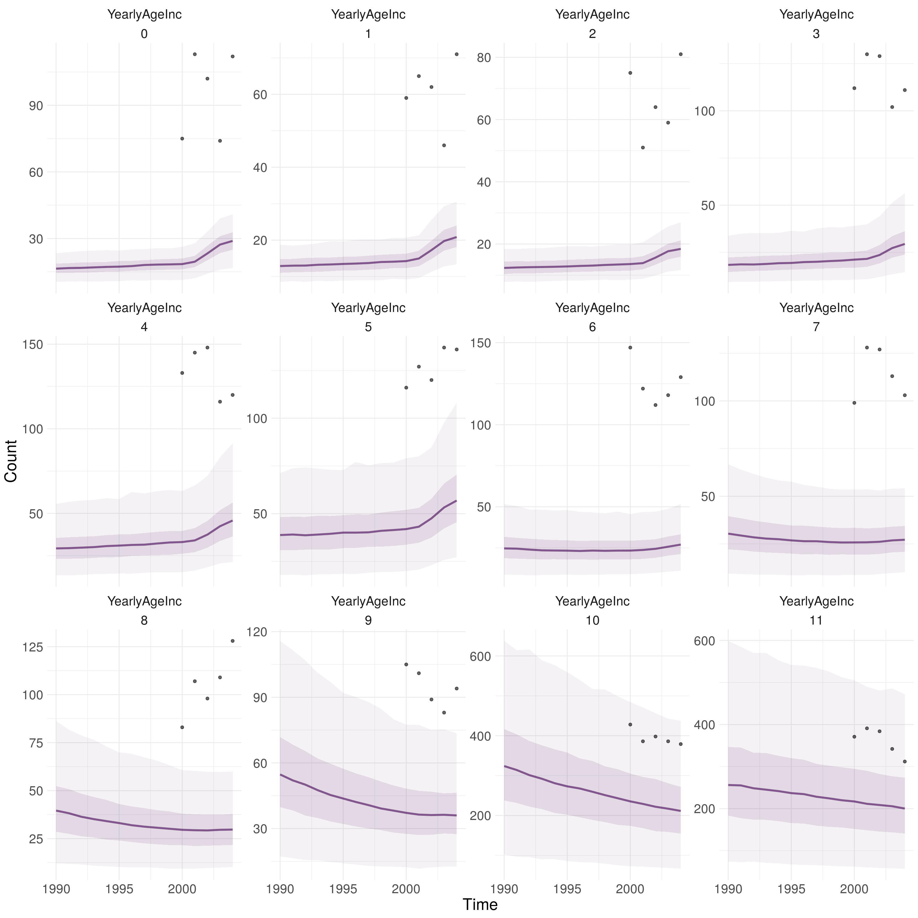
Figure 9.1: Observed and predicted annaul TB incidence stratified by model age group (0-11). 0-9 refers to 5 year age groups from 0-4 years old to 45-49 years old. 10 refers to those aged between 50 and 69 and 11 refers to those aged 70+. The darker ribbon identifies the interquartile range, whilst the lighter ribbon indicates the 2.5% and 97.5% quantiles. The line represents the median. Using 1000 samples from the posterior distribution of the fitted model for the scenario with variability in both transmission and non-UK born mixing.

9.4.5 Posterior parameter distributions

The fitted model had a low effective sample size manifesting in spuriously tight posterior distributions (Figure 9.2; Table 9.4). This indicates that model fitting did not allow for a full exploration of the parameter space. Given that a relatively tight proposal distribution was used this may indicate that an independent proposal is insufficient. It is likely that the key factor behind the model’s consistent under-prediction is the selection of a low value for the current effective contact rate and the historic effective contact rate. It is difficult to interpret these findings further due the low quality of the posterior distribution.

Table 9.4: Prior and posterior medians for fitted model parameters. (95% CrI): 95% credible interval estimated using the 2.5% quantile and the 97.5% quantile. Using 1000 samples from the posterior distribution of the fitted model for the scenario with variability in both transmission and non-UK born mixing.

Parameter	Prior (95%CrI)	Posterior (95%CrI)
\(\beta_{\text{young adult}}\)	5.03 (0.21, 9.68)	7.58 (7.58, 7.58)
\(c_{\text{eff}}\)	1.11 (0.08, 3.04)	0.53 (0.53, 0.53)
\(c^{\text{hist}}_{\text{eff}}\)	10.46 (1.47, 19.41)	1.86 (1.86, 1.86)
\(c^{\text{hist}}_{\text{half}}\)	6.06 (0.48, 15.41)	6.61 (6.61, 6.61)
\(M\)	1.19 (0.09, 3.02)	0.39 (0.39, 0.39)
\(M_{\text{young adult}}\)	5.41 (0.33, 9.77)	8.98 (8.98, 8.98)
\(E_{\text{syst}}\)	0.90 (0.82, 0.98)	0.83 (0.83, 0.83)
\(E_{\text{noise}}\)	0.01 (0.00, 0.02)	0.02 (0.02, 0.02)
\(\iota_{\text{scale}}\)	99.37 (5.55, 194.43)	80.13 (80.13, 80.13)
\(\epsilon^{\text{older-adult}}_L\)	2.01 (1.14, 2.99)	2.11 (2.11, 2.11)

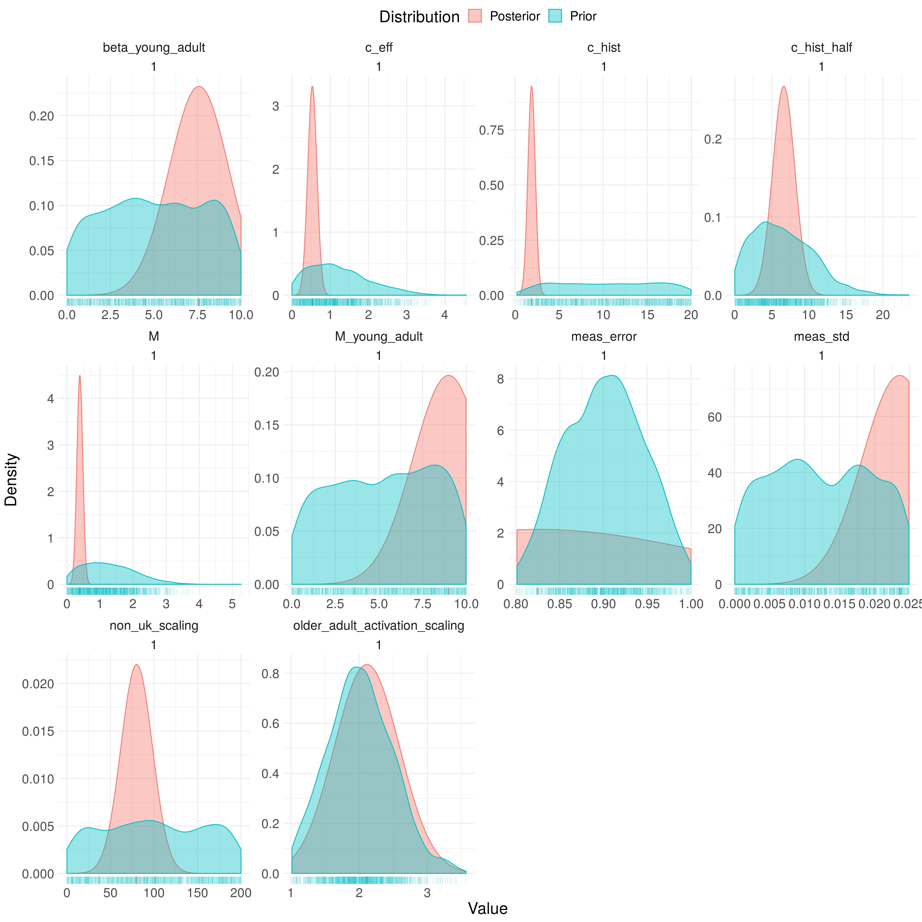
Figure 9.2: Prior and posterior distributions for fitted model parameters. Parameter names in figure are in their coded form. They can be interpreted as the following parameters: \(\beta_{\text{young adult}}\),\(c_{\text{eff}}\), \(c^{\text{hist}}_{\text{eff}}\), \(c^{\text{hist}}_{\text{half}}\), \(M\), \(M_{\text{young adult}}\), \(E_{\text{syst}}\), \(E_{\text{noise}}\), \(\iota_{\text{scale}}\), and \(\epsilon^{\text{older-adult}}_L\). Using 1000 samples from the posterior distribution of the fitted model for the scenario with variability in both transmission and non-UK born mixing.

9.4.6 Parameter Sensitivity

Figure 9.3 shows the partial rank correlation coefficients for each parameter that was fitted to. It indicates that variation in the effective contact rate and non-UK born mixing lead to the greatest variation in TB incidence. Based on the model structure this makes sense as these paremeters are directly linked to modern day transmission. The parameters that modify TB transmission and non-UK born mixing in young adults also lead to significant variation in TB incidence. This corresponds to the findings from the scenario analysis discussed above in which the introduction of these parameters resulted in a greatly improved model fit. The lack of diversity in the posterior distribution seen above means that these findings are indicative only.

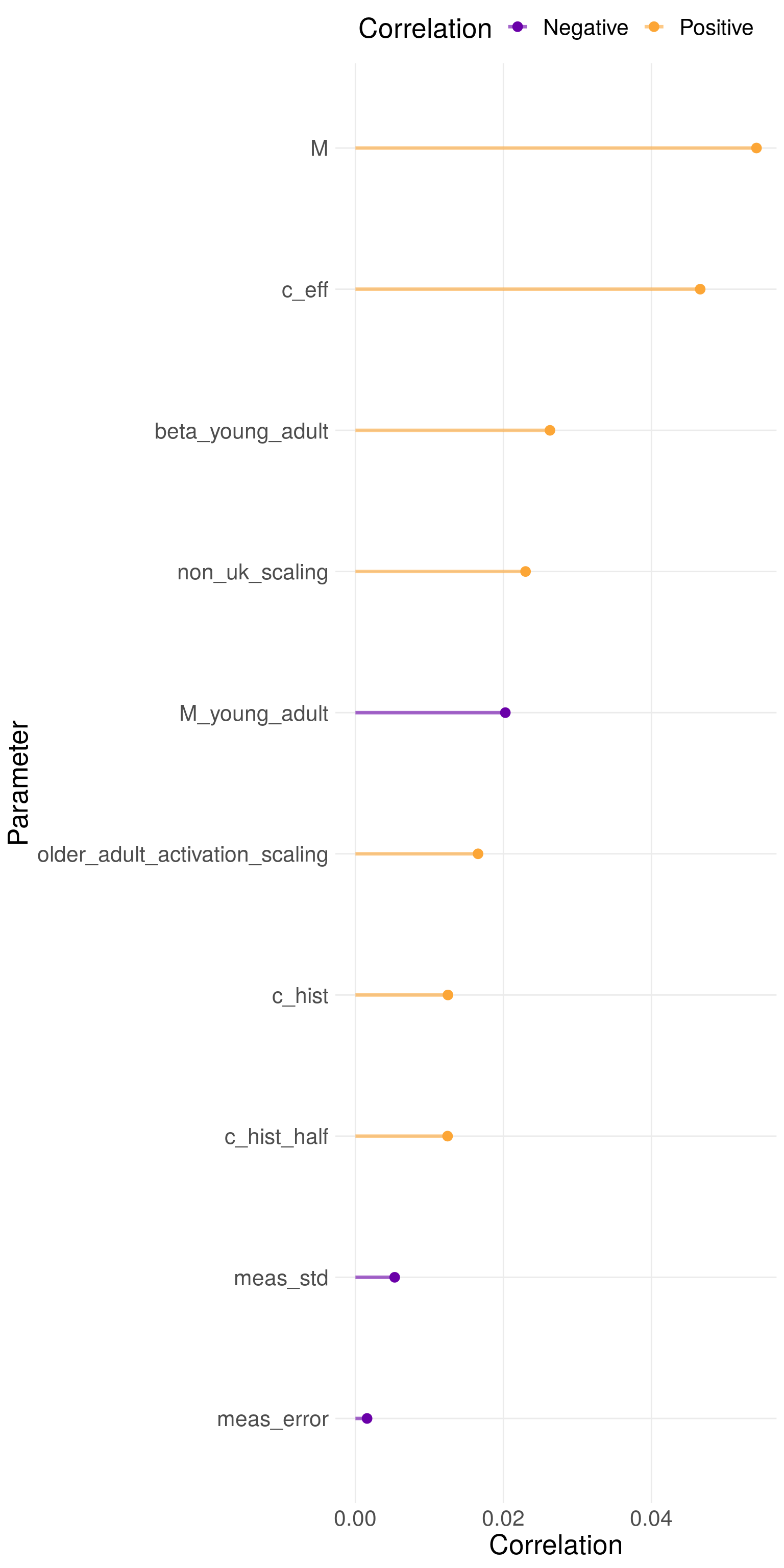
Figure 9.3: Partial rank correlation coefficients for each parameter fitted too. Parameter names in figure are in their coded form. They can be interpreted as the following parameters: \(\beta_{\text{young adult}}\), \(c_{\text{eff}}\), \(c^{\text{hist}}_{\text{eff}}\), \(c^{\text{hist}}_{\text{half}}\), \(M\), \(M_{\text{young adult}}\), \(E_{\text{syst}}\), \(E_{\text{noise}}\), \(\iota_{\text{scale}}\), and \(\epsilon^{\text{older-adult}}_L\). Using 1000 samples from the posterior distribution of the fitted model for the scenario with variability in both transmission and non-UK born mixing.

9.5 Discussion

In this chapter I have formulated the disease transmission model developed in the previous chapter as a state-space model, developed a model fitting pipeline to fit this model to observed data, discussed the approaches taken to try and improve the quality of the model fit, and presented preliminary results from the model fitting pipeline. The model fit the observed data poorly using the approach layed out here. Whilst multiple ad hoc approaches were used to try and improve the quality of the model fit these did little to improve it. The model consistently under-predicted overall TB incidence and also failed to reproduce the observed age distribution. There was little evidence of a good fit to trends over time in the observed data. Model comparison showed that models that included modifying parameters for the transmission probability, and non-UK born mixing in young adults fitted the observed data better than those that did not. The estimated posterior distributions for all parameters were spuriously tight in comparison to the prior distributions. This may be evidence of poor mixing meaning that any conclusions drawn about the parameter sets selected may be incorrect. Parameters that contributed to recent TB transmission dominated those that contributed across the time-span of the model in the parameter sensitivity analysis.

As discussed earlier in this chapter, SMC-SMC was used for all model fitting. This uses an external SMC step to estimate the posterior distribution as well as an internal SMC step to estimate the marginal likelihood. In general, Bayesian model fitting approaches are beneficial as they allow prior information to be fully incorporated into model fitting and they produce posterior distribution estimates rather than point estimates.[123,128] There are two main families of approaches, SMC and MCMC. Using SMC to estimate the posterior distribution has numerous advantages over MCMC. The first of these is that MCMC approaches are sensitive to their initial conditions. If a model has multiple local best fits MCMC may only converge to a single minima rather than fully exploring the posterior distribution. Multiple MCMC chains may be used to try and account for this but as each chain must be independently run to convergence only a few concurrent chains are likely to be practical. SMC on the other hand is initialised with a large sample from the prior distribution, meaning that local minimas are more likely to be explored. Parameter particle weighting and re-sampling then balances the contribution to the posterior distribution of these local minimas based on their fit to the observed data. Additionally, MCMC approaches are by definition sequential,[123] although if they make use of particle filters these can be run in parallel. Increasing the number of particles in a filter may lead to an increase in the chain mixing rate of the MCMC chain but as particles numbers are increased any returns will decrease. To account for this multiple chains are often used, but as outlined above the burn-in required for each chain limits the potential speed-up. In comparison, each SMC parameter particle can have it’s marginal likelihood computed separately. Although the re-sampling step remains a bottleneck as it can only be completed once all marginal likelihoods have been computed. On the other hand SMC is less interactive than MCMC meaning that model fitting is harder to inspect when it is in progress. This is because SMC cannot be inspected sequentually, unlike an MCMC run for which each draw can be inspected as it is computed. Similarly, as SMC is not a sequential technique multiple runs cannot be combined. This means that model fitting must be done in a single run using a priori knowledge to judge the number of MCMC rejuvenation steps required, and the expected total run time. SMC will also have a variable run time based on the effective sample size as rejuvenation only happens when parameter particles have been depleted beyond a certain point. An additional benefit of SMC approaches are that they can theoretically be extended to model selection as well as parameter posterior estimation - effectively estimating posteriors for candidate model structures.[128] Beyond SMC and MCMC there are multiple other model fitting algorithms that each have their own strengths and benefits - discussion of these is outside the scope of this thesis.

The particle filter has been shown to provide an unbiased estimate of the likelihood for arbitrary state-space models.[123] As a full information technique the particle filter provides a more accurate estimate of the likelihood than other approximate techniques with relatively little tuning or user interaction.[123] The major downside of the particle filter is the high compute requirements, with each particle requiring a full model simulation. For highly complex models, the particle filter approach may not be tractable or a reduced level of accuracy of the marginal likelihood estimate must be accepted. In addition, the bootstrap particle filter may become depleted (i.e variance between particles is reduce to such an extent that the effective sample size becomes small) when the model being fitted is a poor fit for the observed data.[123] Whilst this can be resolved using additional particles, or rejuvenation steps, this may not be computationally tractable. There are several alternative particle filters that seek to mitigate these issues but many of them are highly complex and do not significantly reduce the required compute - see [123] for a detailed discussion of some of these alternatives. An alternative approach to the particle filter is to use an approximate technique, such as approximate Bayesian computation (ABC). ABC can be used to avoid having to estimate the likelihood by comparing observed and simulated data.[128] This dramatically reduces the required compute as multiple model simulations per parameter set are no longer required. The comparison between the observed and simulated data is facilitated using a distance function with parameter sets being accepted if they are within some threshold distance. This threshold can be be tuned to produce a good estimate of the posterior distribution. Developing a distance function for all of the observed data can often be challenging so instead the distance is often calculated using a set of summary features.[128] In principle, ABC can be used with a wide variety of algorithms (including a simple rejection approach, MCMC, and SMC) to estimate the posterior distribution but in practice it has been shown that ABC-SMC generally performs better than alternative ABC approaches.[128] The two major limitations of ABC compared to the use of a particle filter is that in most cases summary statistics must be used rather than calculating the distance from the observed data and a function for calculating the distance must be chosen.[128,129] Whilst some techniques exist for evaluating summary statistics the choice is often subjective, relying on domain knowledge.[129] Chosen summary statistics rarely capture the information contained in the observed data fully and can inflate posterior distribution and in the worst cases introduce bias to the estimates.[130] The choice of distance function may also influence the estimates of the posterior distribution.[129]

This chapter showcased the use of LibBi, rbi, and rbi.helpers for fitting a complex transmission model. Unfortunately, the quality of the model fit was poor and the complexity of LibBi makes understanding the root cause difficult. It is possible that the model developed in the last chapter is too complex to be fitted using this approach - at least without the use of several orders of magnitude greater compute resources (or compute time) than available.[123] However, it is also possible that even with these resources this pipeline may not have produced a high quality model fit as the model developed in the previous chapter was clearly much more complex than those envisioned by the developers of the software.[123] Alternatively, the model itself may not be identifiable with the available data.[129] LibBi, rbi and rbi.helpers have great potential as a standardised toolbox for modellers. However, in their current state they are difficult to use beyond relatively simple use cases. This difficulty is compounded by sporadic, inconsistent, documentation of both the underlying software and it’s R interface. On top of this, both LibBi itself and the R libraries that support it have multiple apparent bugs that can be frustrating to debug due to the layered nature of the software. rbi and rbi.helpers are under development and it is likely that many of these issues will be dealt with over time. However, LibBi itself has not had a major release since 2016, the community around it is largely inactive, and it’s complex nature makes it difficult for newcomers to contribute towards it’s development. It is possible that the fitting issues outlined here may be due to errors in the code used to implement the model from the previous chapter. This is unlikely as manual prior tuning has shown that a relatively good fit to the observed data can be achieved with the current model but these results could not be reproduced using the model fitting pipeline. However, this does not mean that the modelling code is bug free. Model bugs, if present, would bias results from the fitted model rather than preventing a good fit to the data or would prevent the model from being manually tuned to fit the data.

There are many other tools available within the R ecosystem for fitting infectious disease models and detailing them all is beyond the scope of this thesis. However, LibBi, rbi, and rbi.helpers represent an attempt to provide a complete modelling framework rather than being a simple toolbox for model fitting. The pomp package has a similar aim making a comparison worthwhile.[10] pomp defines models using a similar structure to that presented here and used within LiBbi. However, rather than using it’s own modelling language it relies on the use of either R or C code. This has several advantages in that pomp models can more easily be generalized, can be understood and implemented by users new to the package and can make use of packages from the wider R and C ecosystem. The downside to this approach is that for complex models the use of C is essentially a requirement for efficiency reasons and implementing complex models in C can be an error prone and time consuming process. pomp offers support for PMCMC, iterated filtering, and ABC-MCMC but does not support SMC based approaches (such as SMC-SMC and ABC-SMC).[10] In developing the work presented here, and in the previous chapter, a simpler model was developed using pomp³⁹. This work was not included in this thesis as it was not sufficiently developed. However, it highlight similar issues with the pomp package to those observed when using LibBi. Whilst pomp’s documentation, stability, and testing were much improved over LibBi it had similar limitations when it came too complex models. This was to such an extent that I developed numerous helper functions to deal with both the input and output of pomp models⁴⁰. pomp’s documentation also has a heavy focus on iterated filtering over other model fitting techniques.

Whilst the results presented here are not encouraging it may be the case that with a greatly extended run-time a better fitting model may be found. The first step to testing this is to rerun the pipeline using several orders of magnitude more rejuvenation steps - as these have no RAM overhead. Even if the resulting model fits are still poor this may indicate areas for improvement - in either the model fitting pipeline or the model itself. Reducing model complexity may also help via decreasing the computational burden, allowing more particles to be used, and also reducing the size of the potential parameter space. Possible simplifications are to remove features, such as the treatment population, that do little to alter the dynamics but are present due to use case concerns or switch from a continous framework to a discrete one. An alternative option is to re-code the model developed in the last chapter into a more generic form (i.e C) and to attempt to fit the model using other techniques that are less compute intensive and more robust - such as SMC-ABC. Another option would be to re-implement the model in the form required by another modelling package - such as pomp. However, this would mean running the risk of again getting stuck within a framework that is difficult to debug and may not be working as expected. A final option would be to reduce the complexity of the model and potentially fit to less complex data. This may be the only solution if the current model is not identifiable.

The model fitting pipeline developed here was theoretically robust, and highly reproducible, but in practice did not produce a high quality model fit. It is difficult to determine whether this was caused by the complexity of the model combined with the high compute requirements of SMC-SMC or if the software implementation itself was at fault. However, LibBi’s high barrier to entry and difficulty of use made both implementing the model, and assessing whether the model fitting was working as expected more difficult. It is likely that a more generic model implementation coupled with a less compute intensive fitting approach would produce more useful results. This work does still have some merit as it pushed both LibBi and SMC-SMC to it’s limits helping to define what the limitations of this approach, and specialised modelling packages more generally, may be. It is possible that with an extended run-time model fits may become more reliable and hence more usable.

9.6 Summary

• Defined the disease transmission model from the previous chapter as a state-space model, outlined the available data to be used for fitting it, and detailed a measurement model to link the observed data with the dynamic TB model.
• Developed a model fitting pipeline based on SMC-SMC to fit the previously defined state-space model to TB notification data. The theoretical background for this approach was outlined as well as the key steps for implementing it in practise.
• As the quality of model fit achieved was poor ad hoc calibration approaches, and the results they gave, were discussed.
• The scenarios outlined in the previous chapter were evaluated using DIC and the implications of the findings were discussed.
• Model forecasts from the best fitting scenario, as established using the DIC, were compared to observed data. Posterior distributions from this model fit were then contrasted with the prior distributions. Finally, parameter sensitivity was estimated using the posterior distributions.
• Discussed the strengths and limitations of the work presented here, as well as outlining potential further work.

References

2 Public Health England. Tuberculosis in England 2017 report ( presenting data to end of 2016 ) About Public Health England. 2017.

9 Funk S, Camacho A, Kucharski AJ et al. Real-time forecasting of infectious disease dynamics with a stochastic semi-mechanistic model. Epidemics 2016;22:56–61.

10 King AA, Nguyen D, Ionides EL. Statistical Inference for Partially Observed Markov Processes via the R Package pomp. Journal Of Statistical Software 2016;69:1–43.

60 Stevenson M, Nunes T, Heuer C et al. epiR: Tools for the Analysis of Epidemiological Data. 2017.

123 Murray LM. Bayesian State-Space Modelling on high-performance hardware using LibBi. Journal of Statistical Software 2015;67:1–36.

124 Jacob PE, Funk S. Rbi: R interface to libbi. 2019. https://CRAN.R-project.org/package=rbi

125 Funk S. RBI.helpers. Published Online First: 2019.https://github.com/sbfnk/RBi.helpers

126 Gelman A. Bayesian Data Analysis: Second Edition. 2004.

127 Marino S, Hogue IB, Ray CJ et al. A methodology for performing global uncertainty and sensitivity analysis in systems biology. J Theor Biol 2008;254:178–96.

128 Toni T, Welch D, Strelkowa N et al. Approximate Bayesian computation scheme for parameter inference and model selection in dynamical systems. Journal of The Royal Society Interface 2009;6:187–202.

129 Lintusaari J, Gutmann MU, Kaski S et al. On the identifiability of transmission dynamic models for infectious diseases. Genetics 2016;201:911–8.

130 Busetto AG, Numminen E, Corander J et al. Approximate bayesian computation. PLoS computational biology 2013;9:e1002803.

---

31. Historic TB notification data via tbinenglanddataclean: https://www.samabbott.co.uk/tbinenglanddataclean/↩

32. See these blog posts for details: https://www.samabbott.co.uk/post/building-an-rstats-workstation/, https://www.samabbott.co.uk/post/benchmarking-workstation-xgboost/, https://www.samabbott.co.uk/post/benchmarking-workstation-benchmarkme/↩

33. Model fitting pipeline R package: https://github.com/seabbs/ModelTBBCGEngland↩

34. Sensitivity code: https://github.com/seabbs/ModelTBBCGEngland/blob/master/R/test_sensitivity.R↩

35. Sensitivity plotting code: https://github.com/seabbs/ModelTBBCGEngland/blob/master/R/plot_sensitivity.R↩

36. Model fitting code: https://github.com/seabbs/ModelTBBCGEngland/blob/master/R/fit_model.R↩

37. Model code: https://github.com/seabbs/ModelTBBCGEngland/blob/master/inst/bi/BaseLineModel.bi↩

38. Thrashing: https://en.wikipedia.org/wiki/Thrashing_(computer_science)↩

39. pomp modle code: https://gist.github.com/seabbs/f08a8a46b1342b8649df963ac015ea31↩

40. idmodelr: https://github.com/seabbs/idmodelr↩